A Complete Guide to IGCSE Graphs
Graphs are an essential part of the IGCSE Math curriculum. They are used to represent data, help visualize trends, and solve complex problems by turning them into visual information. It is essential to know the terminology used to describe different components of a graph. This blog provides you with a comprehensive guide for mastering key graphs.
Key Types of Graphs:
a. Graphs of Linear Equations
Linear equations produce straight-line graphs. They can be expressed in two common ways:
- Equation of a line: y = mx + c
- Function notation: f(x) = mx + c
In function notation, f(x) is simply another name for y. We can read f(x) as “f of x”, meaning “the value of function f at a given value of x”. This notation is useful because it clearly shows the relationship between an input x and its corresponding output f(x). The graph itself is the set of all points with coordinates (x, f(x)).
Tips for Accurate Plotting:
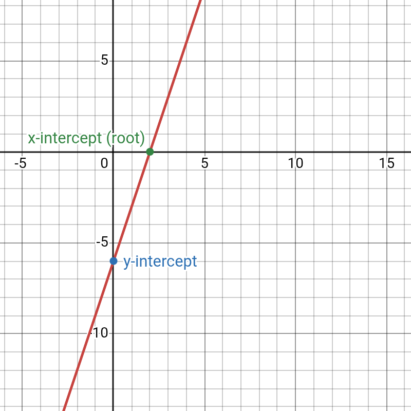
- Find the y-intercept: This is the point where the graph crosses the y-axis. To find it, substitute x = 0 into the function and solve for the output.
- Find the root (x-intercept): This is the point where the graph crosses the x-axis. A linear function has only one root because the highest power of x is 1. To find it, set the entire function equal to 0 and solve for x.
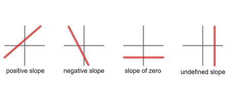
- Gradient (m): The gradient indicates the steepness and direction of the line.
- A positive gradient means the line slopes upwards from left to right.
- A negative gradient means the line slopes downwards from left to right.
- The gradient m is given by the formula m = (y₂ – y₁) / (x₂ – x₁).
Example: Sketch the graph of f(x) = 3x – 6
- 1. Find the y-intercept:
Substitute x = 0:
f(0) = 3(0) – 6 = -6.
The coordinate of the y-intercept is (0, -6). - 2. Find the root:
Set f(x) = 0:
0 = 3x – 6
3x = 6
x = 2.
The coordinate of the root is (2, 0). - 3. Confirm the Gradient:
Using the two points (0, -6) and (2, 0):
m = (0 – (-6)) / (2 – 0) = 6 / 2 = 3.
This confirms the gradient in the function is 3.
b. Quadratic Graphs
Quadratic equations have the general form y = ax² + bx + c. These equations produce parabolic graphs.
Tips for Accurate Plotting:
-
- Shape: The sign of the a coefficient determines the parabola’s direction.
- If a is positive (a > 0), the graph is U-shaped and opens upwards.
- If a is negative (a < 0), the graph is n-shaped and opens downwards.
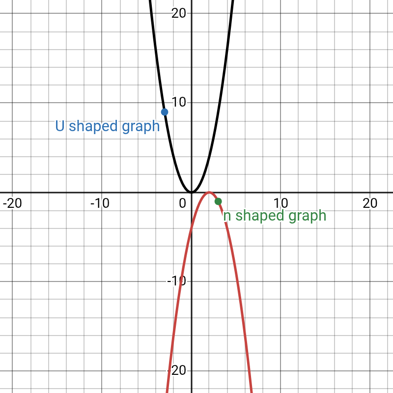
- Shape: The sign of the a coefficient determines the parabola’s direction.
-
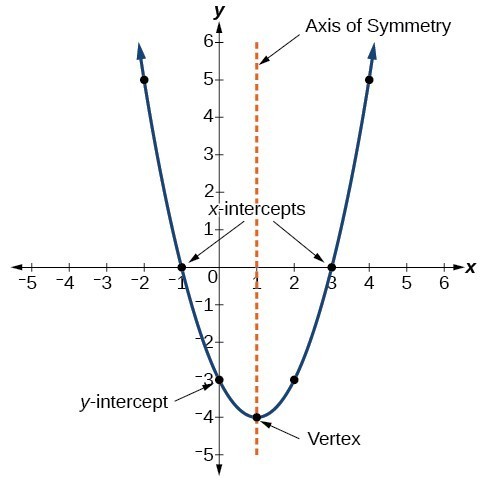
- Y-intercept: Find the point where the graph crosses the y-axis by substituting x = 0. This will always be the point (0, c).
- Roots (x-intercepts): Find the points where the graph crosses the x-axis by setting y = 0. You can solve the resulting quadratic equation by factorizing, using the quadratic formula, or completing the square. A quadratic can have two, one, or no real roots.
- The Vertex: This is the turning point of the parabola.
- If the graph is U-shaped (a > 0), the vertex is the minimum point.
- If the graph is n-shaped (a < 0), the vertex is the maximum point.
- The x-coordinate of the vertex is found using the formula x = -b / 2a. This is a crucial formula to remember. Substitute this x-value back into the equation to find the corresponding y-coordinate.
- Axis of Symmetry: This is the vertical line that passes through the vertex, given by the equation x = -b / 2a.
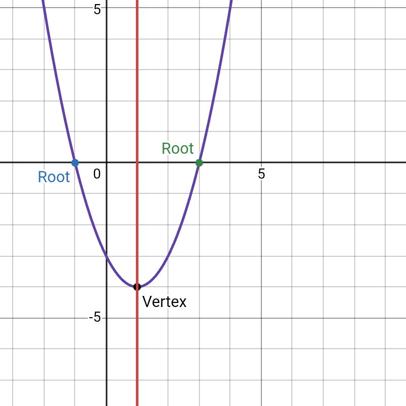
Example: Sketch the graph of y = x² – 2x – 3
- 1. Shape: The coefficient a is 1 (positive), so the graph is U-shaped.
- 2. Y-intercept: Substitute x = 0: y = (0)² – 2(0) – 3 = -3. The y-intercept is (0, -3).
- 3. Roots: Set y = 0: x² – 2x – 3 = 0. Factoring gives (x – 3)(x + 1) = 0. The roots are at x = 3 and x = -1.
- 4. The Vertex: The x-coordinate is x = -(-2) / (2*1) = 1. The y-coordinate is y = (1)² – 2(1) – 3 = 1 – 2 – 3 = -4. The vertex is at (1, -4).
 c. Cubic Graphs
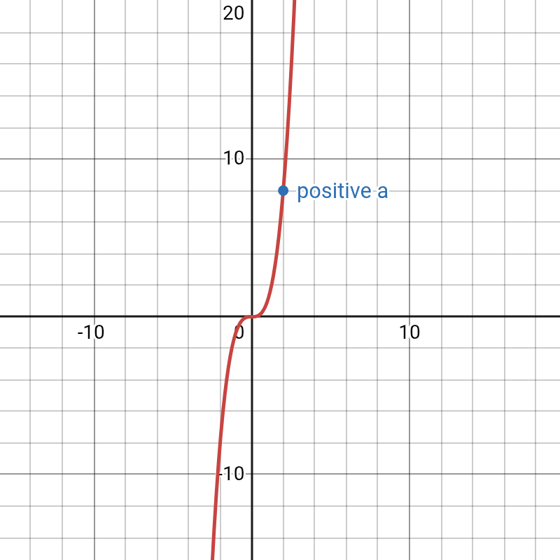
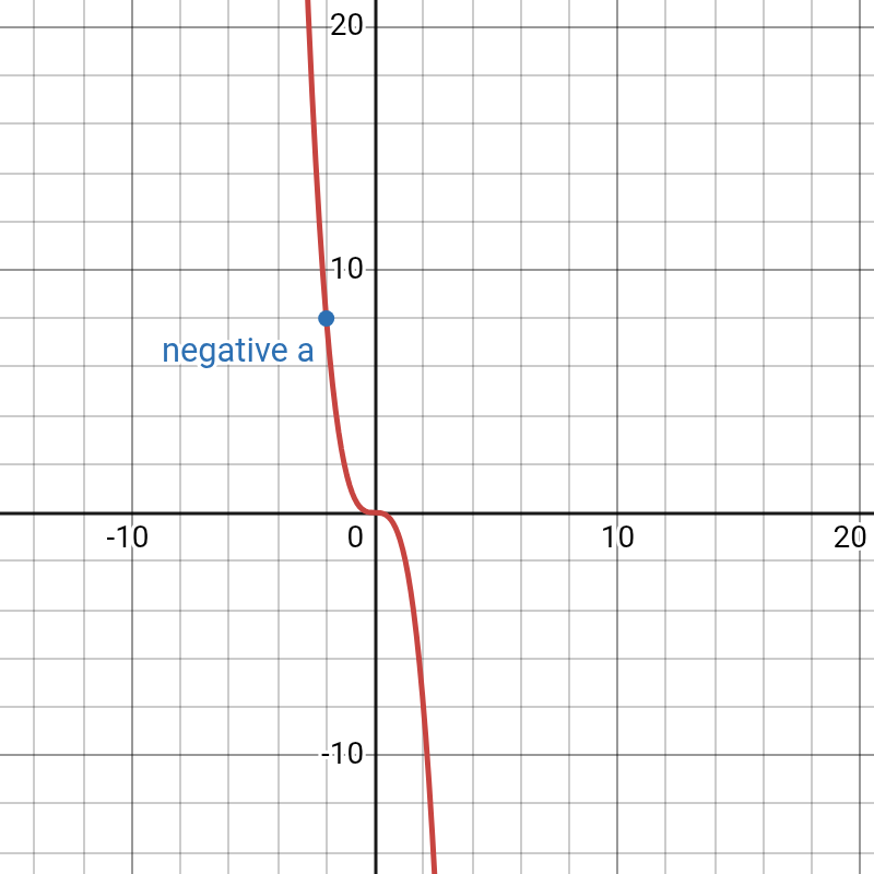
Cubic equations have the general form y = ax³ + bx² + cx + d. Their graphs have a characteristic ‘S’ shape.
Tips for Accurate Plotting:
- Shape: The sign of the a term determines the overall direction.
- If a is positive, the graph generally goes from bottom-left to top-right.
- If a is negative, the graph generally goes from top-left to bottom-right.
- Y-intercept: Find the point where the graph crosses the y-axis by substituting x = 0. This will be the point (0, d).
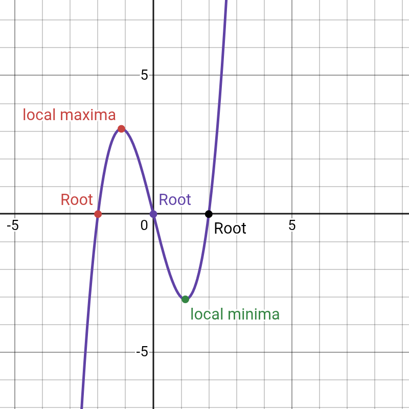
- Roots (x-intercepts): Find the points where the graph crosses the x-axis by setting y = 0. A cubic function can have up to three real roots.
- Turning Points: A cubic graph can have up to two turning points (a local maximum and a local minimum).
Example: Sketch y = x³ – 4x
- 1. Shape: The coefficient of x³ is 1 (positive), so the graph will go from bottom-left to top-right.
- 2. Y-intercept: Substitute x = 0: y = (0)³ – 4(0) = 0. The y-intercept is (0, 0).
- 3. Roots: Set y = 0: x³ – 4x = 0. Factor out x: x(x² – 4) = 0, which further factors to x(x – 2)(x + 2) = 0. The roots are x = 0, x = 2, and x = -2.
 d. Rational Graphs
For IGCSE, rational graphs are typically limited to two main types: the reciprocal graph, y = k/x, and the reciprocal square graph, y = k/x². Both types feature asymptotes, which are lines that the graph approaches but never touches.
Type 1: The Reciprocal Graph (y = k/x)
This graph is a hyperbola with two separate, symmetrical branches. It is identical to the “Reciprocal Graph” section discussed earlier, presented here again for completeness under the broader “Rational Graphs” topic.
Tips for Accurate Plotting:
- Shape and Quadrants: The shape is a hyperbola. The sign of the constant k determines the location of the branches.
- If k is positive, the branches are in the first and third quadrants.
- If k is negative, the branches are in the second and fourth quadrants.
- Asymptotes: The graph is undefined when the denominator is zero, leading to asymptotes.
- Vertical Asymptote: The line x = 0 (the y-axis).
- Horizontal Asymptote: The line y = 0 (the x-axis).
- Symmetry: The graph has rotational symmetry of 180° about the origin (0, 0).
- Key Points: There are no intercepts. Plot a couple of simple points to guide your sketch.
Example: Sketch the graph of y = 2/x
- 1. Shape and Quadrants: The value of k is 2 (positive), so the two branches will be in the first and third quadrants.
- 2. Asymptotes: The asymptotes are the y-axis (x = 0) and the x-axis (y = 0).
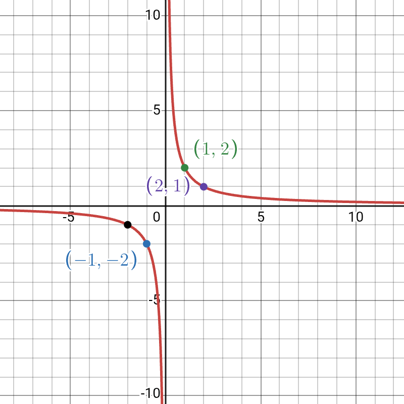 3. Key Points:
- When x = 1, y = 2/1 = 2. Point: (1, 2).
- When x = -1, y = 2/-1 = -2. Point: (-1, -2).
- When x = 2, y = 2/2 = 1. Point: (2, 1).
- When x = -2, y = 2/-2 = -1. Point: (-2, -1).
Type 2: The Reciprocal Square Graph (y = k/x²)
This graph also has two branches, but its shape and symmetry are different from the y = k/x graph.
Tips for Accurate Plotting:
- Shape and Quadrants: The key feature is the x² term in the denominator. Since x² is always positive (for any non-zero x), the sign of y depends only on the sign of k.
- If k is positive, y is always positive. Both branches are above the x-axis in the first and second quadrants. The shape resembles a volcano.
- If k is negative, y is always negative. Both branches are below the x-axis in the third and fourth quadrants.
- Asymptotes: The asymptotes are the same as for the reciprocal graph.
- Vertical Asymptote: The line x = 0 (the y-axis).
- Horizontal Asymptote: The line y = 0 (the x-axis).
- Symmetry: The graph has reflectional symmetry across the y-axis. The part of the graph on the right is a mirror image of the part on the left.
- Key Points: There are no intercepts. Plot points for both positive and negative x values to see the symmetry.
Example: Sketch the graph of y = 2/x²
- 1. Shape and Quadrants: The value of k is 2 (positive), so y will always be positive. Both branches are above the x-axis in the first and second quadrants.
- 2. Asymptotes: The asymptotes are the y-axis (x = 0) and the x-axis (y = 0).
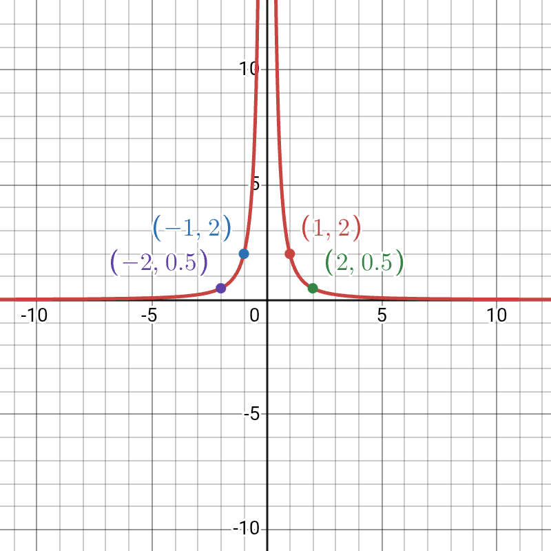 3. Key Points:
- When x = 1, y = 2/(1)² = 2. Point: (1, 2).
- When x = -1, y = 2/(-1)² = 2. Point: (-1, 2).
- When x = 2, y = 2/(2)² = 2/4 = 0.5. Point: (2, 0.5).
- When x = -2, y = 2/(-2)² = 2/4 = 0.5. Point: (-2, 0.5).
- Notice how the y-values are the same for x and -x, confirming the symmetry.
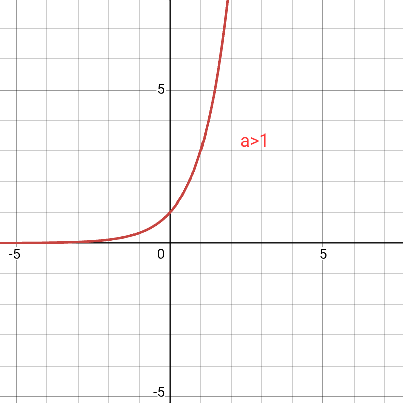
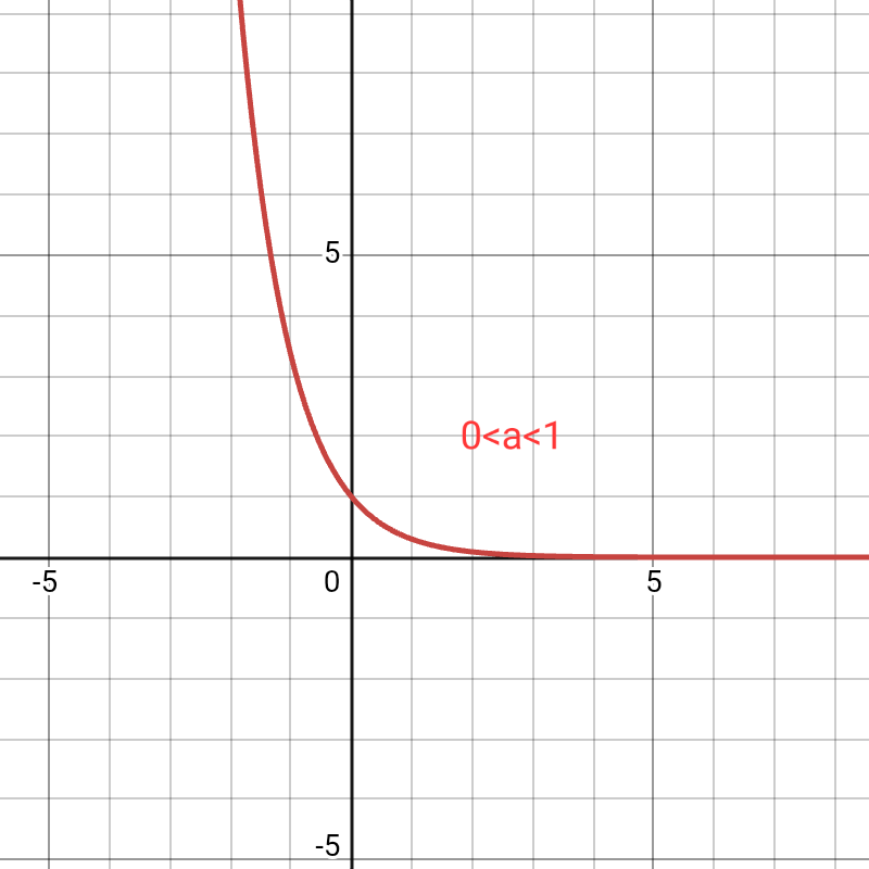
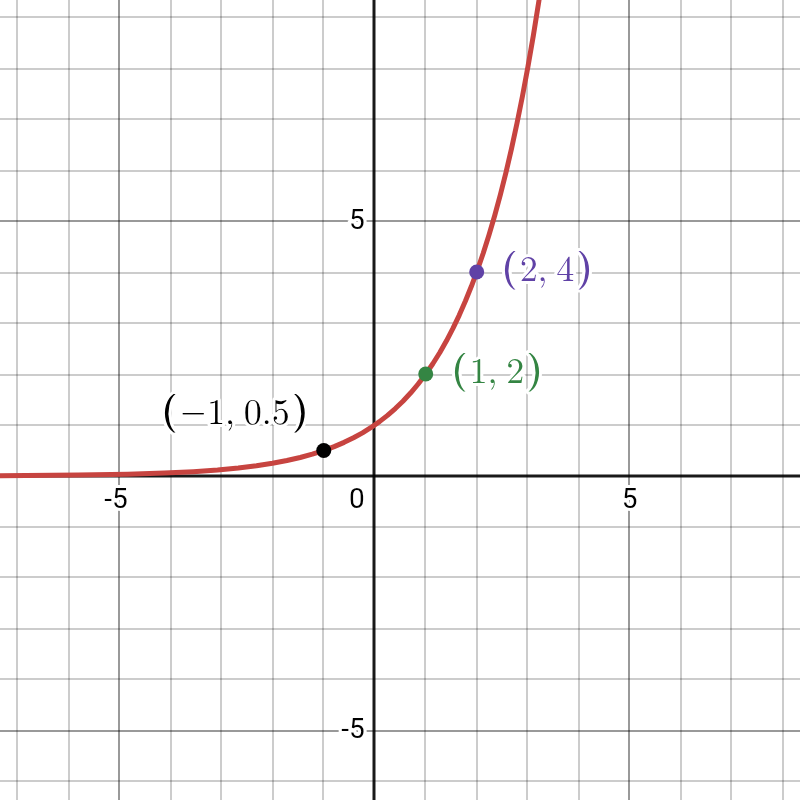
e. Exponential Graphs
Exponential graphs are defined by equations where the variable x is in the exponent, such as y = aˣ. The direction of an exponential graph depends on the base, a.
- Exponential Growth: This happens when the base a is greater than 1 (a>1). The graph rises from left to right, starting slow and becoming progressively steeper. It models things that increase rapidly over time.
 Exponential Decay: This occurs when the base a is between 0 and 1 ( 0 < a < 1). The graph falls from left to right, starting steep and becoming progressively flatter as it approaches the x-axis. It models things that decrease over time, like radioactive decay.
Tips for Accurate Plotting:
- Shape: For a base a > 1, the graph shows exponential growth, rising slowly on the left and very steeply on the right. The entire graph is above the x-axis.
- Y-intercept: Find the value when x = 0. Any number to the power of 0 is 1, so the y-intercept is always (0, 1).
- Asymptote: The graph gets very close to the x-axis on the left side but never touches it. The x-axis (y = 0) is the horizontal asymptote.
- Key Points: There are no roots. To guide your sketch, find the coordinates for a few integer values of x, such as x = 1 and x = 2.
Example: Sketch the graph of y = 2ˣ
- 1. Shape: The base a is 2, which is greater than 1, so the graph shows exponential growth.
- 2. Y-intercept: Substitute x = 0: y = 2⁰ = 1. The y-intercept is (0, 1).
- 3. Asymptote: The horizontal asymptote is the line y = 0.
- 4. Key Points:
- When x = 1, y = 2¹ = 2. Point: (1, 2).
- When x = 2, y = 2² = 4. Point: (2, 4).
- When x = -1, y = 2⁻¹ = 1/2. Point: (-1, 0.5).
 f. Trigonometric Graphs
These are periodic graphs that repeat their shape at regular intervals.
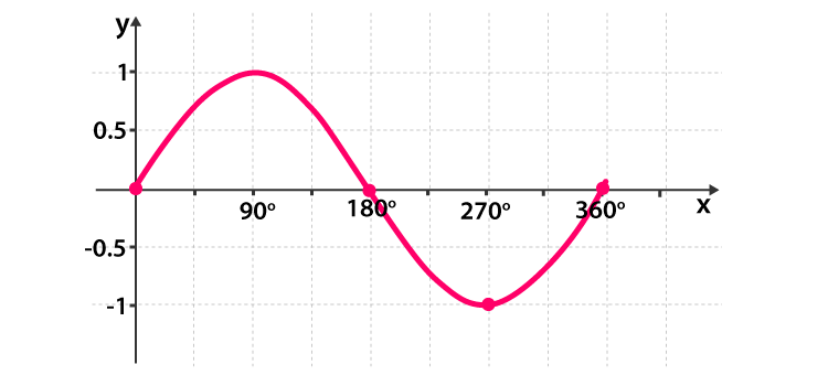
Sine Graph: y = sin(x)
The sine graph is a continuous wave that starts at the origin.
- Period: The graph completes a full cycle every 360°.
- Amplitude: The wave oscillates between a maximum height of 1 and a minimum height of -1.
- Key Points (0° to 360°):
- Crosses the x-axis at 0°, 180°, and 360°.
- Reaches a maximum point (peak) at (90°, 1).
- Reaches a minimum point (trough) at (270°, -1).
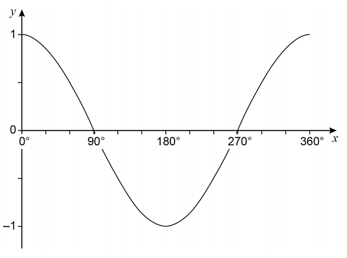
 Cosine Graph: y = cos(x)
The cosine graph is a wave identical to the sine graph but shifted horizontally. It starts at its maximum point.
- Period: The graph completes a full cycle every 360°.
- Amplitude: The wave oscillates between a maximum of 1 and a minimum of -1.
- Key Points (0° to 360°):
- Starts at a maximum point at (0°, 1).
- Crosses the x-axis at 90° and 270°.
- Reaches a minimum point at (180°, -1).
- Ends the cycle at a maximum point at (360°, 1).
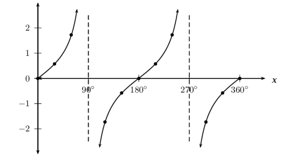
 Tangent Graph: y = tan(x)
The tangent graph is not a continuous wave but a series of separate branches.
- Period: The graph repeats its pattern every 180°.
- Asymptotes: The graph is undefined at certain values, creating vertical asymptotes. These occur at x = 90°, x = 270°, and so on (every 180°).
- Key Points:
- Crosses the x-axis at 0°, 180°, 360°, etc.
- It passes through the origin (0, 0) and increases towards infinity as it approaches the asymptotes.
- Approaches asymptotes at 90° , 270° , etc.
 Common Pitfalls:
1. Before You Plot
- Sign Errors: When substituting negative numbers, always use brackets, like y = (-2)² – 3(-2).
- Wrong Scale: Scan your calculated min/max values first, then choose a scale that fills most of the grid.
- Incomplete Table: Always calculate enough points to clearly see the shape of the graph, especially around turning points.
2. While You Plot
- Messy Drawing: Use a sharp pencil for points and curves, and a ruler for all axes and straight lines.
- “Dot-to-Dot” Curves: Draw smooth, continuous curves through your points; never connect them with a ruler.
- Pointy Parabolas: Ensure the vertex of a quadratic graph is a smooth, rounded turn, not a sharp point.
- Missing Labels: Always label the x-axis, the y-axis, and the graph itself with its equation (e.g., y = 2x + 1).
3. Graph-Specific Mistakes
- Asymmetric Parabolas: Remember a quadratic graph is symmetrical about the vertical line passing through its vertex.
- Reciprocal Graph Errors: The curves must get very close to the axes but never touch or cross them (asymptotes).
- Reciprocal Square (y = k/x²) Errors: If k is positive, both branches must be above the x-axis. x² makes y always positive.
- Trigonometric Graph Start Points: y = sin(x) must start at (0,0). y = cos(x) must start at its peak, (0,1).
- Incorrect Trigonometric Axis: Label the x-axis with angles (90°, 180°, etc.), not standard numbers.
Learning Graphs the All Round Way:
Graphing is considered one of the toughest units in IGCSE Math. At All Round Education Academy HK, we have a team of highly qualified and experienced tutors who with the aid of their knowledge and official IGCSE Examination Questions can help you master Graphing techniques and help you secure a level 9 on your final exams. For more information, please contact us at tuition@allround-edu.com or +852 6348 8744.